In a recent post I have written about a few basic concepts of the Sloan Digital Sky Survey (SDSS) and how to retrieve some data using ADQL from its servers. Now, in this post, I'm going to introduce two major kinds of objects in more depth and explain how to use sdss python library to access and analyse these objects. If you've not yet installed sdss python packege, use can easily install it with pip package manager:
pip install sdss
There are two main classes in this package that we are going to introduce in this article: PhotoObj and SpecObj classes.
In the last post I have already explained the photometric data and the PhotoObj table which can be queried via SQL Search. Alternatively, you can use PhotoObj class from the sdss python package by passing the identifier of the object to this class. In the photometric data, a unique ID has been assigned to each object in the sky, called ObjID. After creating the instance of the class, you will have access to some of its attributes and methods:
import sdss

ph = sdss.PhotoObj(1237648720693755918)

print(ph.objID)
print(ph.downloaded)
print(ph.sky_version)
print(ph.rerun)
print(ph.run)
print(ph.camcol)
print(ph.field)
print(ph.id_in_field)
Output:
1237648720693755918
False
2
301
756
2
427
14
The value of ph.downloaded is False, which means that the data for this object has not been downloaded from the SDSS server. We have to call the download method in order to have access to other attributes and methods:
ph.download()

print(ph.specObjID)
print(ph.downloaded)
print(ph.ra, ph.dec)
print(ph.type)
print(ph.mag)
Output:
320932083365079040
True
179.689293428393 -0.454379058425512
GALAXY
{'u': 19.09722, 'g': 17.60256, 'r': 16.82659, 'i': 16.43768, 'z': 16.14087}
Note that if the object has spectrum, the specObjID attribute will return a non-zero number that will be explained in the next section. The type attribute may return one of the three values UNKNOWN, GALAXY or STAR, based on the image processing algorithm implemented by the SDSS.
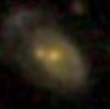
Another useful information is the image of the object. If you want to view the object, simply call the show method. You can pass scale, width and/or height arguments if you want.
ph.show()
Output:
Another possibility is to get the image data as a numpy array. To do this, call the cutout_image method:
img_data = ph.cutout_image()
print(img_data.shape)
Output:
(300, 300, 3)
Again, if you want different scale and resolution, you can pass scale, width and/or height arguments when calling the cutout_image method.
Another major type of data in the SDSS, is the spectroscopic data. A unique ID, called specObjID is assigned to each one-dimensional spectrum. You can create an instance of the SpecObj class by passing the specObjID of your desired object. After creating the instance, you have access to some of its attributes and methods.
To resume our example, let's pass the specObjID we've got above:
sp_id = sp.specObjID

sp = sdss.SpecObj(sp_id)

print(sp.specObjID)
print(sp.downloaded)
print(sp.plate)
print(sp.fiberID)
print(sp.mjd)
print(sp.run2d)
Output:
320932083365079040
False
285
184
51930
26
In order access to other methods and attributes, you should first download the spectrum by calling the download method.
sp.download()

print('Photo objID:', sp.bestObjID)
print('Downloaded:', sp.downloaded)
print('ra:', sp.ra)
print('dec:', sp.dec)
print('Spec Type:', sp.type)
print('Mag:', sp.mag)
print('Redshift:', sp.z)
print('Main Class:', sp.mainClass)
print('Sub Class:', sp.subClass)
Output:
Photo objID: 1237648720693755918
Downloaded: True
ra: 179.68928
dec: -0.45436733
Spec Type: GALAXY
Mag: {'u': 19.09722, 'g': 17.60256, 'r': 16.82659, 'i': 16.43768, 'z': 16.14087}
Redshift: 0.09484052
Main Class: GALAXY
Sub Class: STARFORMING
Note that the bestObjID is the corresponding objID of the object in the photometric data.
After creating the instance of the SpecObj class, you can retrieve the spectrum of the object in three ways.
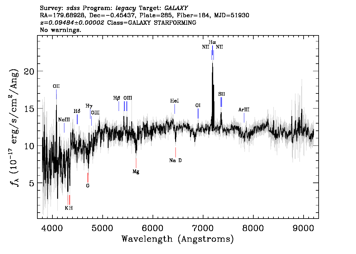
The simplest way to view the spectrum is by calling the show_spec method. The plot of the spectrum with be shown as an image. This is the plot that SDSS has created. If you want just see the spectrum without having control on the data, this is the most straightforward way.
sp.show_spec()
Output:
I you want the values of flux for each wavelength, you can use the spec_df method. This method will return a pandas DataFrame with four columns: Wavelength, Flux, BestFit and SkyFlux. The Flux column is the raw data as recorded by the spectroscope, while the BestFit column is the result of the SDSS algorithms.
df = sp.spec_df()
print(df)
Output:
      Wavelength    Flux  BestFit  SkyFlux
0       3801.019   4.973    7.549    5.208
1       3801.893  11.402    7.506    5.351
2       3802.770   4.585    7.430    5.252
3       3803.645   7.782    7.438    5.225
4       3804.522   8.624    7.160    5.252
...          ...     ...      ...      ...
3834    9189.672  11.865   11.371    4.139
3835    9191.786  10.487   11.460    4.010
3836    9193.905  10.810   11.474    3.982
3837    9196.020  12.317   11.527    4.032
3838    9198.141  12.533   11.609    4.075

[3839 rows x 4 columns]
If you want full control, you should download the spectrum as a FITS file using the download_spec method. This method has a few optional arguments such as path and filename in the case if you want to save the downloaded spectrum in a specific folder and with a specific name. Furthermore, this method, by default, will download a lite FITS file, but you can change this behavior with the lite and fits arguments.
Let's just download the spectrum of our example as a lite FITS file in the current working folder and with the default filename:
sp.download_spec()
Now, If you look at your working directory, you will find the downloaded file: spec-0285-51930-0184.fits.
In another post, I will discuss about the contents of this file, the way we can analyse it and create a nice spectrum plot from it.