In this page I introduce two kinds of astronomical Python packages. First, the most popular and useful libraries that can be used in astronomical calculations. Second, the libraries that I have created for this reason. I will update this page as I find another useful library or if I create a new library or make major changes in the existing ones. I don't mention here general packages such as pandas, numpy, matplotlib, scipy, sklearn and keras, as you can easily find a lot of tutorials about them on the Internet. All the packages I introduce in this page can be installed using pip package manager.
There are an increasing number of astronomical python packages and I can't and don't want to introduce all of them. I'm going to talk about just the most important one, astropy which is essential and indispensable for astronomical data science. I also mention a few libraries that can be helpful.
I've never seen an astronomical library more comprehensive than astropy. It is created by great teams and is very well documented. It consists of several modules for dealing with time, coordinates, tables, quantities, models, etc. Some of its functionalities make your everyday life really easy, such as using constants, unit conversions and handling FITS files.
Let me show you just a few of its general applications in everyday life. Physical quantities have two parts: unit and value. For example, when we say that the speed of light in vacuum is 299792458 m/s, we are talking about a quantity, speed, which has two parts: its unit is metres per second and its value is 299792458. You can define create this quantity in astropy as follow:
>>> from astropy import units as u
>>> speed = 299792458 * u.Unit('m/s')
>>> print(speed)
299792458.0 m / s
One advantage of creating quantities with units, is that you can convert them to other units using .to() method. Let's find the speed of light in km/h:
>>> print(speed.to('km/h'))
1079252848.8 km / h
Another useful module in astropy is constants. Let me show it with an example. We want to find the Newtonian gravitational force between the Earth and the Sun:
We can create each of these quantities as explained above, but the constants module have already defined them and I we have to do is importing them from this module:
>>> from astropy.constants import G, M_earth, M_sun, au
>>> f = G * (M_earth * M_sun) / au**2
>>> print(f)
3.541545424043141e+22 kg m / s2
The resulting unit is kg m / s2 which is newton. Remember \(F=m a\), or if you want to be sure convert it to newton directly with .to() method:
>>> print(f.to('N'))
3.541545424043141e+22 N
You can find other useful constants here.
The most popular python package for querying astronomical databases is certainly astroquery, which is a coordinated package of astropy. There are a large number of web forms and databases supported by this library. Maybe the most important feature of this package is the compatibility of its data formats with astropy, as in the case of tables, units and etc.
Another astropy compatible library is astroplan. It can be useful for those who are interested in observational astronomy.
This python package has come with a nice textbook which explains step-by-step useful methods and technics you can use in astronomical analysis. The package helps you specially in creating machine learning models. There are a lot of interesting datasets you easily download using astroML.datasets module.
As an astro data scientists, you may find that you are repeating some procedures that you can't find already implemented in a published library. You may also encounter a situation that think the existing implementations are not sufficiently efficient for what you want to do. In these cases you decide to create and publish your own library. This is the reason why I have created the following libraries.
My initial object when I created this package was retrieving data from NASA's JPL HORIZONS System, which is a great tool for getting positions and velocities of the solar sytem objects. It has been implemented in horizons module. This module has two classes, Vector and Observer, to return positions. I have given examples of using this module here.
Another useful module is catalogues that can be used to retrieve data from a specific catalog. There's a python dictionary in this module which returns name and decription of existing astronomical catalogs in the current version of the package. First, you have to create an instance of the Catalogue class, by passing the catalog's name. There are some optional arguments as well: columns determine which columns should be returned, n_max is the maximum number of rows to be returned, where and order_by as used as SQL clauses. Once you've created an instance of the class, you can access its attributes and methods. Use columns attribute to find out which columns will be returned in the current instance. To know all possible columns in the table, use available_columns() method. Finally, use download() method to retrieve data from the server.
Let's get data of very bright objects, whose apparent magnitude is less than 1, from the Hipparcos Catalog:
>>> import hypatie as hp
>>> hip = hp.Catalogue(name='hipparcos', where='Vmag > 1')
>>> data, meta = hip.download()
>>>
>>> data.shape
(15, 12)
>>>
>>> data.head()
     HIP    _RA_icrs   _DE_icrs  Vmag  ...    B-V  Period  HvarType    SpType
0  24608   79.172329  45.997991  0.08  ...  0.795     NaN         U  M1: comp
1  69673  213.915300  19.182410 -0.05  ...  1.239     NaN         U    K2IIIp
2  91262  279.234735  38.783692  0.03  ... -0.001     NaN         U    A0Vvar
3  32349  101.287155 -16.716116 -1.44  ...  0.009     NaN         U    A0m...
4  37279  114.825493   5.224993  0.40  ...  0.432     NaN              F5IV-V

[5 rows x 12 columns]
The cosmology has a parent classes, CosModel, to help you create a cosmological model of universe. To use the standard model with predefined data from Planck 2018 data release, you can create an instance of Plank18, which is a child class of CosModel. You can find several examples of using this module in some of our blog posts, such as Hubble's Law and How to calculate Scale Factor.
Some useful function have been created in transform module that can help you in coordinate transformations. Two important functions in this module are radec_to_altaz and altaz_to_radec to transform between ICRS and Altitude-Azimuth coordinates.
The package will be updated and you can find out the version you've installed by calling __version__. There is still much task to be implemented, and of course, pull requests are welcome.
If you're interested in deep-sky astronomy, you should learn how to retrieve data from Sloan Digital Sky Survey. There are different ways for this reason, but sdss python package has made it really simple for you. I've written a series of posts on this topic, so here I don't go into details. You can create a Region class by passing the coordinates of its center and a field of view to get the image of that part of the sky. You can also find different kinds of objects in that region.
There are also two other essential classes, PhotoObj and SpecObj. Each of theses object can be created by passing objID and specObjID, repectively. You can start learning about SDSS along with using the sdss python package here.
You should know ELODIE/SOPHIE archives if you're interested in stellar spectroscopy. These archives, provided by Observatoire de Haute-Provence, consist of spectra of stars recorded across time and are presented in FITS format. The stelspec library makes it easy to access data and download spectrum of stars from these archives.
To get data from each of these archives, you should create an instance of the archive's corresponding class, Elodie or Sophie by passing star's name. Once you've created an instance, you have access to its methods. Currently, there are three methods: .ccf(), .spec() and .get_spec(). Each of the first two methods returns a table as pandas DataFrame, Cross-Correlation Functions table and Spectra table. The third method, .get_spec(), downloads a FITS file, which is one of the available spectra of the star. You should determine which one should be returned by passing required arguments to this method.
Let's say we want to see available spectra of the star HD217014 in the ELODIE archive and download one of them. We create an instance of Elodie and use .ccf() to see existing spectra.
>>> from stelspec import Elodie
>>> el = Elodie('HD217014')
>>> ccf = el.ccf()
>>> ccf.shape
(153, 12)
>>>
>>> ccf.head()
   datenuit imanum  imatyp         jdb  ...    vfit sigfit  ampfit  ctefit
0  19940914   0022  OBTH    49610.5268  ... -33.260  4.800  0.1738  0.9996
1  19940916   0017  OBTH    49612.4657  ... -33.229  4.802  0.1737  0.9997
2  19941027   0008  OBTH    49653.2973  ... -33.226  4.768  0.1739  0.9995
3  19941029   0009  OBTH    49655.3067  ... -33.286  4.773  0.1754  0.9999
4  19950110   0007    OBTH  49728.2289  ... -33.321  4.764  0.1764  0.9990

[5 rows x 12 columns]
As you see, there are 153 spectra for this star in the ELODIE archive. The date and exact time that each spectrum has been recorded are given in datenuit and jdb columns, respectively. The radial velocity calculated from each spectrum is given in vfit column. To download a spectrum you should pass its and datenuit to imanum. Let's download the first spectrum to the working directory:
>>> # download spectrum as FITS file
>>> el.get_spec(19940914, '0022')
If you're interested in astrodynamics, you can try gravitational python pachakge, wich is a N-body simulation library. You should first create an instance of the Simulation class, then create body objects using add_body method. Finally, you can you use run method to run the simulation, or just use play method to show the animated simulation.
from gravitational.simulation import Simulation

# create Simulation object
sim = Simulation()

# Add first body
b1 = sim.add_body(name='Star',
                  color='y',
                  size=25,
                  mass=2e30,
                  position=(0, 0),
                  velocity=(0, 0))

# Add second body
b2 = sim.add_body(name='Planet',
                  color='b',
                  size=10,
                  mass=6e24,
                  position=(1.5e11, 0.5e11),
                  velocity=(0, 20000))

# play the simulation
sim.play(dim='2d', path=True)
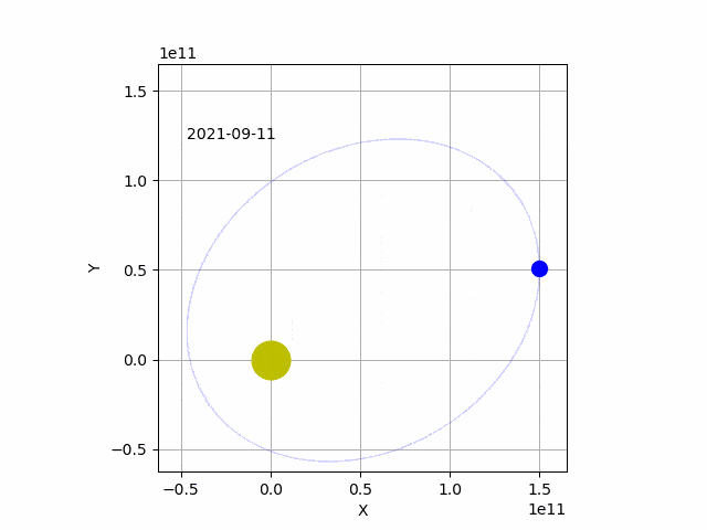
You can add as many bodies as you wish to the simulation. The Simulation has some useful mehtods that can help you in astrodynamics calculations and simulations. Fr example, by passing two body objects to set_orbit method, it will change the velocity of the small body in order to set it in the orbit of the larger body. Another method, set_lagrange, helps you to put a body (such as a sattelite) in one of the five lagrangian points of another body (a planet for axample), with respect to a third body (such as a star).